Life Cycle Strategy - Life Cycle and Degradation Strategies
Configure a Life Cycle
- While viewing a Life Cycle Strategy, select the 'Life Cycle' tab:
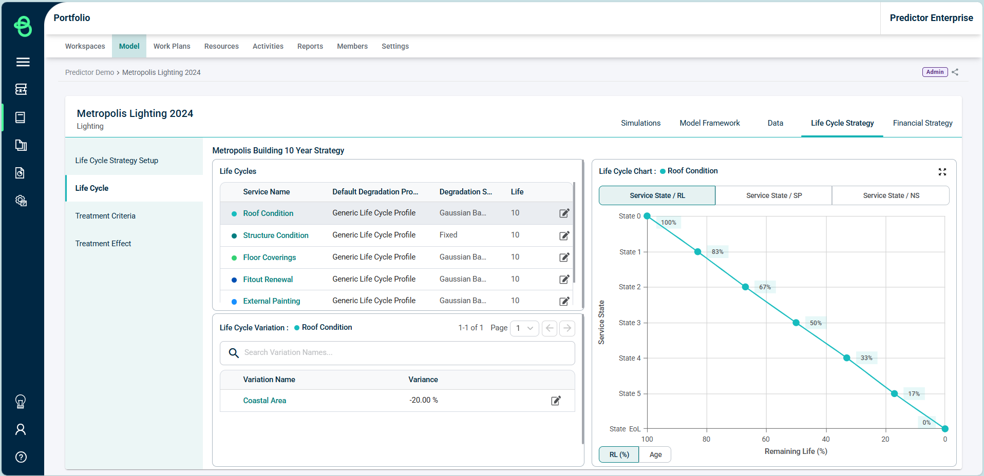
- Select the edit
 icon next to a life cycle.
 - Select the Degradation profile to use in the drop-down in the life-cycles box:
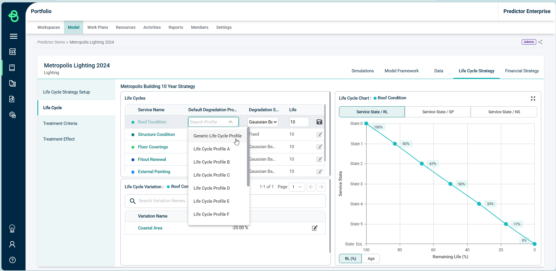
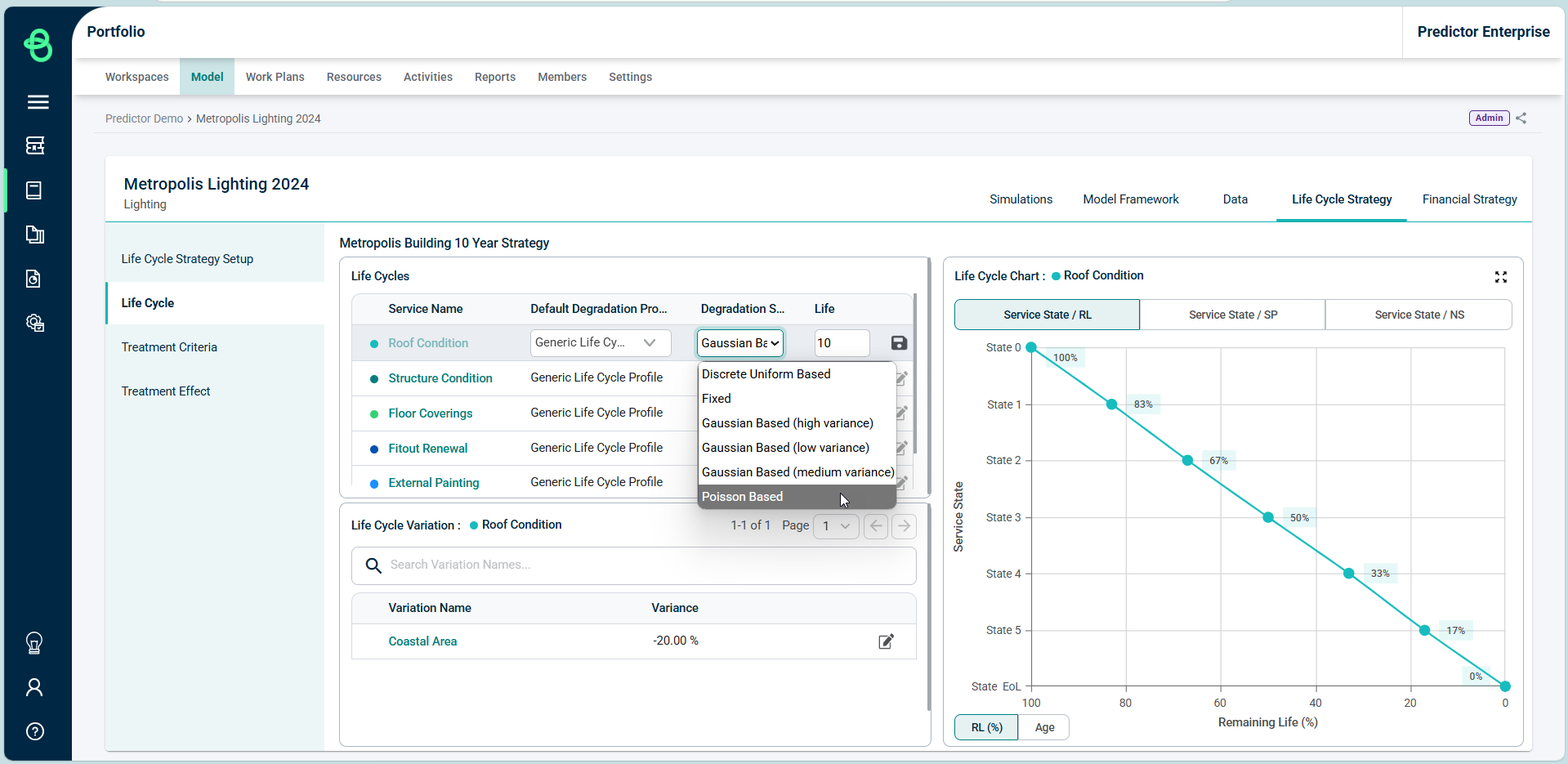
- Select the Degradation Strategy to use in the drop-down in the life-cycles box:
The Default Life field specifies the value for the useful life for that Service Criteria for any Asset which does not have a useful life value mapped for that Service Criteria during the Data Import. The Default Life can be manually set. The minimum Default Life for any Service Criteria is 6 years.
Degradation Strategy
When modeling infrastructure assets over time, we need to determine the event of how each asset degrades over its lifecycle path and whether that event is random or fixed in time.
In the Degradation Profile article, we discussed how a degradation profile describes the relationship between remaining useful life, remaining service potential and native scaling (typically assigned to specific service states).
The Degradation Profile has a direct relationship to the Degradation Strategy, which informs the algorithm when and how assets will degrade between service states.
For example, we assign the following degradation profile (ignoring the service potential % and native scale for the time being) to reflect how our assets within our model will degrade over time, assigning the below profile to our asset service criteria.
| Service State | Remaining Life (%) |
| 0 | 100 |
| 1 | 83 |
| 2 | 67 |
| 3 | 50 |
| 4 | 33 |
| 5 | 17 |
| 6 (EoL) | 0 |
If we now inform the model that our assets have a 100-year useful life, Brightly Predictor will generate what is termed ‘degradation points’ using the service state / remaining life % relationship.
The following degradation point profile is defined below and used by the Predictor algorithm to degrade each asset within your model dataset:
| Service State | Age / Degradation |
| 0 | 0 |
| 1 | 17 |
| 2 | 33 |
| 3 | 50 |
| 4 | 67 |
| 5 | 83 |
| 6 (EoL) | 100 |
In our Life Cycle Strategy, if age is the sole variable that explains how an asset degrades over its Life Cycle path, then we can determine the exact point of any individual service criteria and how the asset will degrade during the simulation. This can be achieved by using the Fixed Degradation Strategy in Predictor. This method will degrade all assets from one service state to the next at precisely the year determined by their Life Cycle chart. This will result in all similar assets degrading at the same point in time, rather than being spread out over a range of time.
Using our previous example, the Fixed Degradation Strategy when utilised will always degrade 100% of assets assigned with a service state 0 to service state 1 at year 17 and from service state 1 to service state 2 at year 33 and so on, reaching end of life by year 100 exactly.
What if the Life Cycle is not a Fixed Event?
In the world of predictive infrastructure modelling (particularly for long life infrastructure like pavements, facilities, under-ground pipes, rail, side-walks, buildings and structures, bridges, tunnels etc), the behaviour of degradation over time is not a fixed event, but rather a random event.
The outcome of a random event cannot be determined before it occurs, but it is very likely that it can be one of several possible outcomes. The way that assets behave cannot be predicted with certainty, although based on historical behaviour, as asset practitioners, we notice that there is regularity with regards to how assets degrade over time.
Therefore, in the case of long life infrastructure assets, the Life Cycle is a path that a service criteria will degrade on predominantly expected averages. By applying theories of probabilities we can also assign what is termed as frequencies around these degradation points, to reflect that not all assets on average will move between these degradation points at the exact assigned degradation point.
It is this frequency that is reflected via the application of the probability distribution profiles (Degradation Strategies) that reflect the number of events that occur in a given interval of time.
In Predictor, this behaviour is implemented by using different degradation strategies when generating the degradation point, which are:
- Poisson Based Degradation Distribution: Predictor’s Simulation will use a Poisson distribution to degrade assets over a range of time.
- Gaussian Degradation Distribution (high variance): Predictor’s Simulation uses a Gaussian distribution, also known as the Normal distribution, to degrade assets probabilistically over a range of time. The high variance setting is typically more suitable for longer life infrastructure.
- Gaussian Degradation Distribution (medium variance): Predictor’s Simulation uses a Gaussian distribution, also known as the Normal distribution, to degrade assets probabilistically over a range of time. The medium variance Distribution is the default setting.
- Gaussian Degradation Distribution (low variance): Predictor’s Simulation uses a Gaussian distribution, also known as the Normal distribution, to degrade assets probabilistically over a range of time. The low variance setting is typically more suitable for assets with a short life.
- Discrete Uniform Based Degradation Distribution: Predictor's Simulation will degrade the same percentage of assets from one condition to the next over a range of time, resulting in a similar number of assets degrading each year.
The following diagram identifies the comparison plot (using our earlier degradation profile example) of these degradation strategies when determining the service state versus age relationship.
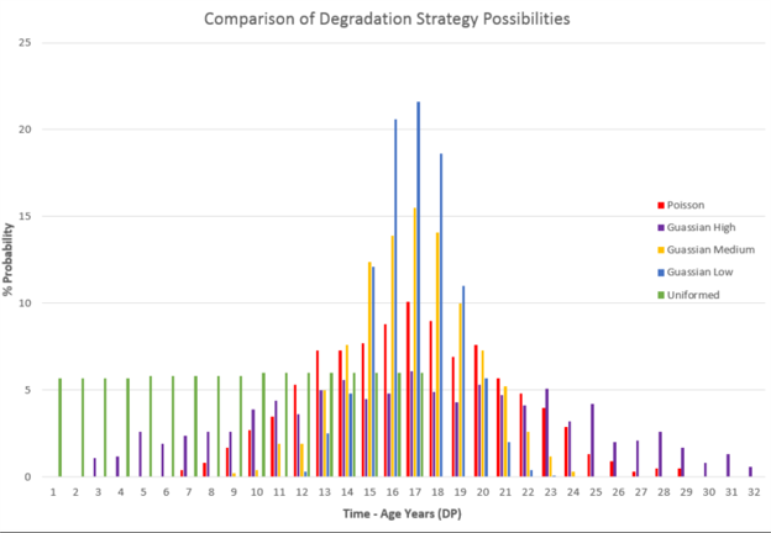
If we apply the Poisson Distribution Strategy, 10.1% of assets assessed as service state 0 will now transition to service state 1, compared to 6.1% for the Gaussian High Variance Strategy and 15.5% for the Gaussian Medium Variance Strategy and 21.6% for the Gaussian Low Variance Strategy, all at year 17.
Each method then applies different frequencies which see for example 1.1% of assets in service state 0 transition to service state 1 at year 3 if we use the Gaussian High Variance method. This method also sees 1.7% of assets transitioning to service state 1 not at year 17, but at year 29.
Hence each method applies different probabilities with regards to the required degradation point (age) that an asset needs to attain, prior to deteriorating to the next service state.
Which method is most appropriate?
As a benchmark derived from thousands of analyses, the default degradation strategies recommended are the Gaussian Medium Variance or Poisson methods as these tend to better reflect the fact that no assets on average will degrade at the mean degradation point and that whilst some assets tend to degrade earlier, there are others that will tend to take longer, this reflects how long life infrastructure assets behave.
As further information is compiled by organisations with regards to how assets behave within their environments, this data can be used to improve degradation strategy selection when modeling.
How do we assign Degradation Strategies?
Degradation strategies can be assigned to individual service criteria. For example, if we were using asset condition and asset age as two separate service criteria, we can now assign the Gaussian Medium Variance Strategy to the service criteria representing the asset condition and Fixed Strategy to the service criteria representing age.
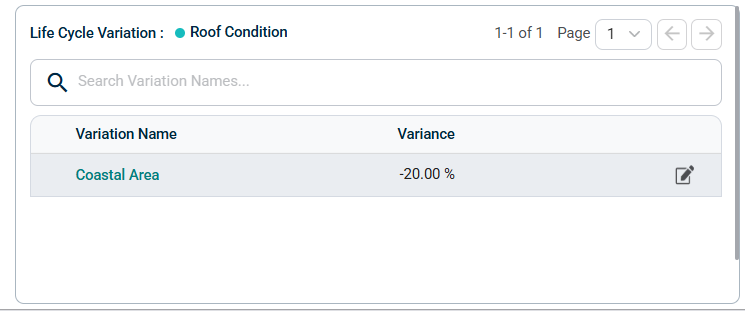
Life Cycle Variation
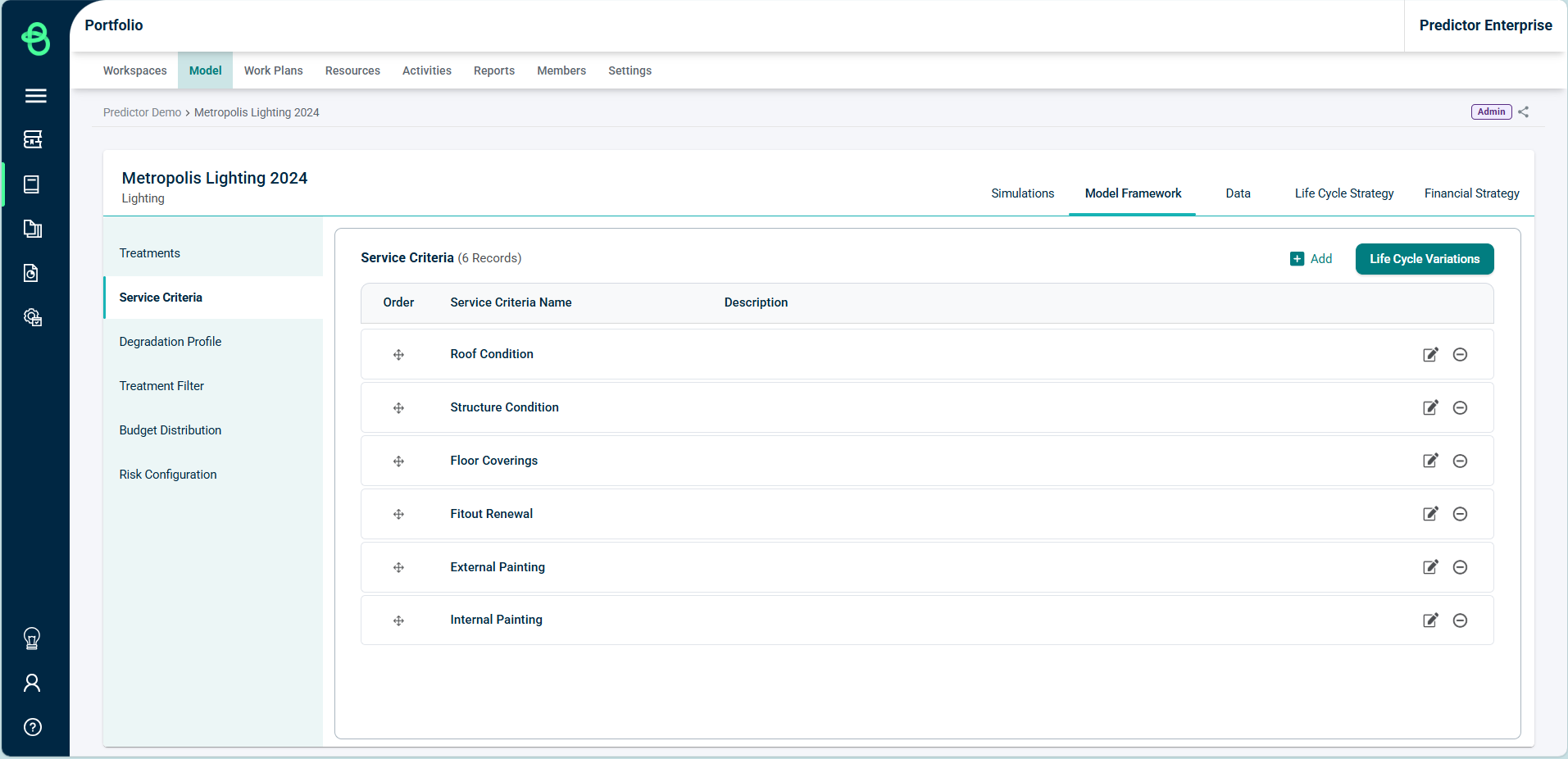
A new Life Cycle Variation can be added by selecting the ‘Life Cycle Variation’ button in the Service Criteria tab of the Model Framework section.
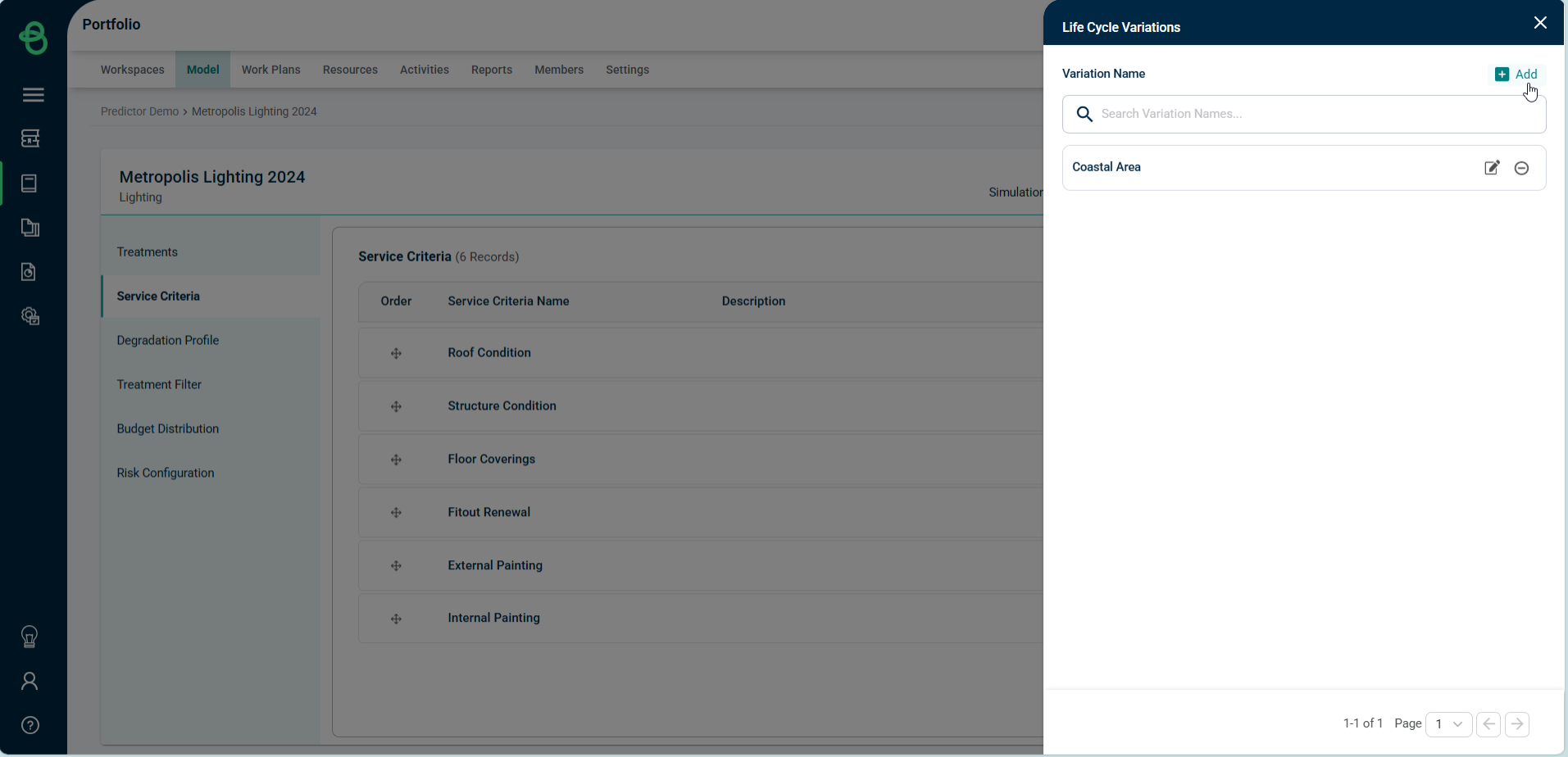
If the data imported into the Model contains Life Cycle Variation fields, then labels provided in the template will appear in the 'Life Cycle Variation' box in the Life cycle tab of the model.
It can then be configured to apply a modifier to the degradation curve based on each asset's service criteria, where a variance of less than 0% decays faster, while a variance above 0% will increase the Life Cycle by that additional percentage, meaning it will have a long life. For example, the Life Cycle Variation can be configured such that an asset in a coastal area degrades 20% faster: